w2clustertable: a way to track storm properties over time

w2segmotionll provides a way to identify storm cells and track their properties over time so as to data mine storm attributes.  But w2segmotionll is not the best place for that functionality because:

  1. w2segmotion is also used to estimate motion from clusters, so as to create image nowcasts (using w2advector).  Adding storm attribute generation makes w2segmotion a performance hog in real-time applications.
  2. Storm tracking should not be limited to w2segmotion’s way of identifying clusters. Any object-identification method (not just the enhanced watershed approach we use) should be supported.

Following the WDSS-II philosophy, therefore, the cluster-table functionality of w2segmotion has been split off into a new program called w2clustertable.  Instead of providing the -X option to w2segmotion, pass the XML file into the -X option of w2clustertable.

w2clustertable also takes, as input, a label grid (the “KMeans” output of w2segmotion) and motion estimates (the Motion_East and Motion_South) outputs of w2segmotion.  But you could also use w2imgmotion to obtain cross-correlation-based motion estimates. And you can use any scheme to create a labeled set of storms (1,2,3…) to get their properties. It is not necessary for storm#4 in one frame to be storm#4 in the next frame (i.e., w2clustertable will associate storms using centroid-match or overlap or one of several built-in association methods).

If you use w2clustertable, please continue to cite our 2009 J. Tech paper:  V. Lakshmanan and T. Smith, “Data mining storm attributes from spatial grids,” J. Ocea. and Atmos. Tech., vol. 26, no. 11, pp. 2353-2365, 2009


With this change, here are some related programs in the storm identification and tracking realm:

  1. w2segmotionll uses K-Means clustering and Enhanced Watershed to identify storm cells at multiple scales.
    (see: V. Lakshmanan, K. Hondl, and R. Rabin, “An efficient, general-purpose technique for identifying storm cells in geospatial images,” J. Atmos. Oceanic Technol., vol. 26, no. 3, pp. 523-37, 2009)
  2. w2segmotionll uses these storms to compute motion estimates  (see: V. Lakshmanan, R. Rabin, and V. DeBrunner, “Multiscale storm identification and forecast,” J. Atm. Res., vol. 67, pp. 367-380, July 2003.)
  3. w2segmotionll and w2clustertable can both be used to track storm cells over time (see: V. Lakshmanan and T. Smith, “An objective method of evaluating and devising storm tracking algorithms,” Wea. Forecasting, vol. 25, no. 2, pp. 721-729, 2010.), but w2clustertable is now preferred.
  4. w2segmotionll and w2clustertable can both be used to compute storm attributes but w2clustertable is now preferred. (see: V. Lakshmanan and T. Smith, “Data mining storm attributes from spatial grids,” J. Ocea. and Atmos. Tech., vol. 26, no. 11, pp. 2353-2365, 2009)
  5. w2segmotionll and w2advectorll can both be used to create nowcasts of other fields from motion estimates obtained by tracking storms on one field but w2advectorll is the preferred way to do that. (see: V. Lakshmanan, R. Rabin, and V. DeBrunner, “Multiscale storm identification and forecast,” J. Atm. Res., vol. 67, pp. 367-380, July 2003.)
  6. w2flatten will take the multiscale cluster table output by either w2segmotionll or w2clustertable and “flatten” it into a single table, to make multi-scale data mining possible (forthcoming paper by Humphrey, Lakshmanan, Smith, Smith and Thompson).


Tags: None

Merge radars into 3D Mosaic

Written by Bryan Burlingame [Part 3 of How to Create Reflectivity -10C]

Creating Cache for the Desired 3D Latitude and Longitude Grid

Create the cache for the 3D latitude and longitude grid to be utilized for all the radars using createCache. This will create a storage of data that the w2merger process (to be run later) can access. The information in the cache is relating to the size of the domain you wish to use, as well as which radars will be on that grid. The default directory for this cache is in your $HOME directory, and is titled .w2mergercache.

        1. The process of creating the cache MUST BE DONE FOR ALL RADARS, here is an example of the command

createCache -o $HOME -i KXXX -T /path/to/terrain/KXXX.nc -t “50 -111 20” -b “27 -93 1” -s “0.05 0.05 1” –verbose

    1. o = creates the cache called “.w2mergercache in the $HOME directoy. w2merger will look in the $HOME directory for the cache, so best to leave it at $HOME (default is $HOME)

    2. i = the radar the cache is being created for (e.g. KXXX) MUST BE DONE FOR ALL RADARS

    3. T = the path to the terrain files so any terrain obstructions for a radar will be known. . You can obtain these data, if you do not already have them, from ftp://ftp.nssl.noaa.gov/users/lakshman/conus_radar_blockage.tgz.

    4. t = Top (and NW corner) of the of the new lat lon grid being created.

    5. -t “50 -111 20” -b “27 -93 1” -t “(north-Lat) (west-Lon) (vertical levels)”

    6. b = Bottom (and SE corner) of the of the new lat lon grid being created.

    7. -b “27 -93 1” -b “(south-Lat) (east-Lon) (lowest vertical level)”

    8. s = The spacing done between the grid points

      1. -s “0.05 0.05 1” -s “(Lat spacing) (Lon spacing) (vertical level spacing (km))”

  1. MUST BE DONE FOR ALL RADARS, new radars will be added into the first cache created.

    1. *THE –t –b –s variables used must be the same that are passed when using w2merger below

Merging Radar Data to Common Lat/Lon 3D Grid and Interpolating Reflectivity to the -10˚C Isotherm in RAP/RUC Data

The next 3 commands need to be run simultaneously, and in the order specified. This will merge the radar data and will also interpolate it to the RAP data (The shell script I created ran w2simulator in the background, sleep for 2 seconds, then started w2merger and w2segmotionll and worked). After you begin the simulator, it will prompt you to begin other algorithms; at this time, begin the w2merger and w2segmotionll.

  1. w2simulator– This is the command that synchronizes the process and will read in all the various radar directories (AND THE RAP code_index.xml mentioned above), and output the data into index_N.fam directories which are used as the input for the w2merger.

    1. N corresponds to the number of files read into the simulator, one is created per file.

w2simulator -i “/path/to/radar1/code_index.xml /path/to/radar2/code_index.xml /path/to/more/radars/code_index.xml  /path/to/rap/code_index.xml” -o /path /simulation -b 20130515-000258 -e 20130515-010700 –verbose

    1. i = is the path to the radar xml files, and should also include the path to the RAP .xml file created using nse

    2. o = is the output path for where the code_N.fam files are put.

      1. This is the input path for w2merger

    3. b = beginning time of the simulator

    4. e = end time of the simulator

      1. Both –e and –b must be of the format (YYYYMMDD-HHMMSS)

  1. w2merger– This is the command that pulls in the radar and RAP data from the various sources and merges it together onto the grid that was created using createCache. Note that the input in w2merger is the output from w2simulator.

w2merger -i “$COMMON/simulation/index_0.fam $COMMON /simulation/index_1.fam $COMMON /simulation/index_2.fam” -o $COMMON/merged -I ReflectivityQC:00.50 -M $COMMON/segmotion -e 60 -C 5 -t “50 -111 20” -b “27 -93 1” -s “0.05 0.05 1” -a Isotherms –verbose

  1. i = is the path to radar/RAP files that were created by running the w2simulator command. This should be same path as output path of w2simulator, linking to the index_N.fam files in that directory.

  2. o = is the out path of the now merged files (Should be used as input into w2segmotionll)

  3. I = (capitol i) is the variable you wish to merge (eg. ReflectivityQC:00.50 is the quality controlled 0.5 degree reflectivity)

  4. M = tells the merger to refer to and include the output from w2segmotionll. w2merger and w2segmotionll work together in a feedback process.

  5. e 60 = to make an output once every 60 seconds. Doing it without the -e option will cause a rapid update grid that your I/O hardware may not be able handle properly.

  6. C 5 = changes the way data values are combined if they overlap in both space and time. 5 (TimeAndDistanceWeighted) means that the overlapped data are weight with respect to both distance and time so that later data are weighted higher. This is the “common” selection

  7. t –b –s =SAME AS createCache. For meaning of these arguments, refer back to #8 (e-g). The values should be the same as the grid created in this step.

  8. a = to specify the algorithms you wish to run on the 3D grid.

  1. w2segmotionll– This will get motion estimates from the data and feed it into w2merger. Optional, but was recommended within the user guide for multiple radar cases. It corrects for time differences between radar elevations scans (from the same or different radars) by advecting older data before blending.The output directory should be specified in w2merger by passing the –M flag.

w2segmotionll -i $COMMON /merged/code_index.fam -o $COMMON /segmotion -T MergedReflectivityQC -O 5 –verbose

  1. i = is the input path for the code_index.fam directory. This is created by the w2merger command (-o in w2merger). Although it is a directory, when entering the path in the w2segmotionll command, do not have the / at the end.

  2. o = is the output path of the motion estimates, once again is the same as the –M flag passed in w2merger

  3. T = this flag tells the w2segmotionll command what variable to take the motion estimates from.

  4. O = changes the time interval over which motion is computed. If O = 30, then frames at least 30 minutes apart are used in the motion estimation.

Tags: None

Creating QCed Radar Data

Written by Bryan Burlingame [Part 2 of How to Create Reflectivity -10C]

NEXRAD NCDC Data:

Download individual NEXRAD radar data from:

http://www.ncdc.noaa.gov/nexradinv/map.jsp

Or in bulk from:

http://has.ncdc.noaa.gov/pls/plhas/HAS.FileAppRouter?datasetname=6500&subqueryby=STATION&applname=&outdest=FILE

Once downloaded, untar and unzip any files if necessary. Then same as mentioned above organize the files so that only the files you actually need are in a directory.


Converting NEXRAD Level II Data to WDSS-II NetCDF

The steps below need to be done individually for all the radars that you plan to merge (i.e., If you have data from 3 radars, you must run ldm2netcdf (below) 3 times, once for each radar.)

I recommend reading the “quick usage” guides that are available via the WDSS-II website, or typing just the command into the terminal to see the other flags that can be passed. Below explains only the flags which we used.

        1. The command needed to convert the NEXRAD data to WDSS-II NetCDF is ldm2netcdf. An example of the command issued is below.

ldm2netcdf -i /path/to/NEXRAD/data -a -1 -p KXXX -s KXXX -o /path/to/radar/NetCDF/ –verbose

          1. i = input radar directory (where the radar data were downloaded to)
          2. a = reads old LDM files in the input directory
          3. –1 = (one) Not real time
          4. p = pattern recognition.. aka the radar site identifier (e.g. KXXX)
          5. s = the radar site (e.g. KXXX)
          6. o = the output directory (where you want your now NetCDF files to go, if directory does not exist, one will be created for you).
        1. Use replaceIndex to create the needed configuration file code_index.xml.

replaceIndex -i /path/to/code_index.fam -o /path/to/code_index.xml

          1. i = path should the same as the output directory from ldm2netcdf, linking to the code_index.fam/ directory generated by that command
          2. o = should be the same path as the input here, except the output is code_index.xml

De-Aliasing NEXRAD Level II Velocity Data

In this step we will De-alias the radar velocity data.

        1. The command used in this step is “dealias2d.” Here is an example of the command issued.

dealias2d -i /path/to/code_index.xml -o /path/to/radar/files -R KXXX –verbose

  1. i = path should the same as the output directory from replaceIndex ran in the previous step, linking to the code_index.xml file which is the configuration file for all the radar data
  2. o = should be the same output path as used above in ldm2netcdf.
  3. R = should be the same as the flag passed for –p –s in ldm2netcdf (e.g. KXXX)
        1. Run replaceIndex on the code_index.fam directory in your NetCDF output directort. The command issued should be identical to the command issued after running ldm2netcdf. This will update the configuration file so it contains the newly de-aliased velocity data.

Quality Controlling NEXRAD Level II Reflectivity Data

This step will run Quality Control (QC) tests on the radar data to eliminate any noise and clutter. There are two different commands that can be used, and it depends on whether or not your radar data contains dual-pol.

  1. QC the radar data using w2qcnn if you are using radar data that does not contain dual-polarization information or use w2qcnndp if using data that does contain dual-polarization information.
  2. For w2qcnn, here is an example command:

w2qcnn -u -i xml:/path/to/code_index.xml -V Velocity -E /path/to/terrain/KXXX.nc -R 0.25×0.5×460 -o /path/to/radar/NetCDF –verbose

  1. For w2qcnndp, here is an example command:

w2qcnndp -i xml:/path/to/code_index.xml -V Velocity -E /path/to/terrain/KXXX.nc -R 0.25×0.5×460 -s KRRR -o /path/to/radar/files – verbose

  1. u = creates virtual volumes (necessary for w2qcnn; do not use for w2qcnndp)
  2. i = path should the same as the output directory from replaceIndex ran in the previous step, linking to the code_index.xml file which is the configuration file for all the radar data
  3. V = Velocity – tells the program to use dealiased (rather than aliased) velocity in quality control
  4. E = (path) – tells the program where terrain data for each radar may be found for use in quality control
  5. R = 0.25×0.5×460 – tells the program that super-resolution Level II radar data is being quality controlled; if super-resolution Level II radar data are not being utilized, then set this to 1x1x460
  6. S = KRRR – provides the radar site identifier to the program
  7. o = path to the output file directory, should be the same output path as used above in ldm2netcdf and dealias2d.
  1. Run replaceIndex on the code_index.fam directory in your NetCDF output directort. The command issued should be identical to the command issued after running ldm2netcdf and dealias2d. This will update the configuration file so it contains the newly QC’d data.


Tags: None

Getting RUC/RAP data into WDSS-II

Written by Bryan Burlingame [Part 1 of How to Create Reflectivity -10C]

To start, the first steps require the requesting, and downloading of large datasets. This process can be time consuming in both waiting for the NCDC order to come through, and also in downloading the data.

RAP/RUC Data:

Download RAP/RUC from:

http://nomads.ncdc.noaa.gov/data.php?name=access#hires_weather_datasets

After downloading the needed RAP data, organize the data into directories so that only the times you want processed are in a directory. The WDSS-II program reads in whole directories worth of data at a time. So to minimize the processing time, and also the size of your data, only keep the data need for the time of interest. Utilities such as wgrib or wgrib2, available from NCEP, are particularly useful for this task.

Converting RAP/RUC Data to WDSS-II NetCDF

There are two different processes for grib1 data and for grib2 data. Typically, RAP data will be in grib2 format and RUC data will be in grib1. In order for WDSS-II to read in RAP/RUC data, it needs to be in the WDSS-II NetCDF format. Below are the steps needed to convert both GRIB 1 & 2 to the required format.

GRIB 1

  1. The command used to convert GRIB 1 to WDSS-II NetCDF is gribToNetcdf. Here is an example of the command:

gribToNetcdf -i /path/to/grb1 -o /creates/new/directory/NetCDF -k -a -1 -p 2013 -t “50 -111” -b “27 -88” -s “0.03 0.03” –verbose

    1. i = input directory of the GRIB 1 data.
    2. o = where you want the generated NetCDF files to go (creates directory if it DNE).
    3. k = tells command NOT to delete the original GRIB 1 files after processing.
    4. a = if on, will read the existing files in the directory on startup.
    5. -1 = if on, will execute just once (not real-time).
    6. p = pattern recognition (if all files start with rap_130… you would use –p rap_130)
    7. t = the northwest corner of the domain you wish to use (Should be same as below with w2merger).
    8. b = the southeast corner of the domain you wish to use (Should be same as below with w2merger).
    9. s = the horizontal spacing of the domain
  1. Run “replaceIndex” to make a .xml file from .fam directory. The code_index.fam will be the same as the outputDir specified in the griddataingest.xml file you copied over and edited.

replaceIndex -i /path/to/code_index.fam -o /path/to/code_index.xml

  1. i = input directory (path to code_index.fam/) of now WDSS-II NetCDF files (same as output directory used above in gribToNetcdf ).
  2. o = same directory as above, however the output is code_index.xml rather than .fam
  1. Run “nse” to create various products that RAP/RUC does not have, but which WDSS-II needs to interpolate to the various Isotherms in the RAP/RUC data.

nse -i xml:/path/to/code_index.xml -o NSE/ -3 –verbose

GRIB 2

  1. There are two options for converting GRIB 2 to the WDSS-II NetCDF. Option 1 (the recommended option) is to continue onto step 2 below. The other option is to convert the GRIB 2 data to GRIB 1 using the command: cnvgrib –g21 <inputfile> <outputfile>
    1. cnvgrib readme: http://www.nco.ncep.noaa.gov/pmb/docs/grib2/download/cnvgrib.readme
    2. After converting to GRIB 1, revert back to the previous section for converting GRIB 1 to WDSS-II NetCDF.
  1. For GRIB 2, use the WDSS-II Java package to convert GRIB 2 to WDSS-II NetCDF. In steps (a.) and (b.), make sure the proper paths are declared.
    1. export JAVA_HOME=”/usr/bin”
    2. export WDSSII_INSTALL_DIR=”/path/to/wdssii/wdssiijava”
  1. Next you need to copy the file wdssiijava/example/griddataingest.xml into a directory of your choice, and rename it rap.xml or ruc.xml (any name .xml works). Next, edit the newly copied .xml file. At the top of the file change the inputDir to where your data are, and outputDir to where you want it to go. Also change the filenamePatterns to match some part of your input files (if all files start with rap_130… you would use rap_130 as your filenamePattern). You also will want to uncomment the listVariables entry and set it to true.


  1. Now run the following command:

w2java.sh org.wdssii.ncingest.GridDatasetIngest /path/to/copied/griddatasetingest.xml

  1. This will create your configuration file, varList.xml. This file contains all of the meteorological variables in your RAP/RUC data. By editing this file you can change which variables are processed in the new NetCDF files.
  1. Next, edit griddatasetingest.xml that you copied and renamed so to set listVariables to false.
  1. Now run the following command: (Yes, same as above)

w2java.sh org.wdssii.ncingest.GridDatasetIngest /path/to/copied/griddatasetingest.xml

  1. Run “replaceIndex” to make a .xml file from .fam directory. The code_index.fam will be the same as the outputDir specified in the griddataingest.xml file you copied over and edited.

replaceIndex -i /path/to/code_index.fam -o /path/to/code_index.xml

    1. i = input directory (path to code_index.fam/) of now WDSS-II NetCDF files (same directory as outputDir mentioned above).
    2. o = same directory as above, however the output is code_index.xml rather than .fam
  1. Run “nse” to create various products that RAP/RUC does not have, but which WDSS-II needs to interpolate to the various Isotherms in the RAP/RUC data.

nse -i /path/to/code_index.xml -o /path/to/NSE/ -3 –verbose


Tags: None

Interpolating Reflectivity to -10C Level in RAP/RUC Data

Written by Bryan Burlingame

WDSS-II Guide to Interpolating Reflectivity to -10˚C Level in RAP/RUC Data

The process of obtaining data from multiple radars, quality controlling the data, merging the various radars to a common three dimensional latitude and longitude grid, and then interpolating that radar reflectivity to the -10˚C level found in RAP/RUC data is explained here. This process was conducted and then this document created by Bryan Burlingame (burling6@uwm.edu) and Dr. Clark Evans  at the University of Wisconsin-Milwaukee for the purpose of identifying Convective Initiation (CI) in hours immediately following Mesoscale Predictability Experiment (MPEX) research flights.


Lak’s note:

The entire document is being posted in three pieces for easier searchability.  The steps to create the Reflectivity-10C product are:

  1. Get RUC/RAP data into WDSS-II
  2. Create QCed radar data from Level-II
  3. Mosaic radar data taking into account temperature level

Thanks to Bryan for sending me these instructions.


Tags: None

Using GMMs to score gridded forecasts with w2scoreforecastll

Determining how closely a forecast matches what happens in reality is a crucial step in the evaluation of any type of forecast. Gridded forecasts, which are of particular interest to WDSS-II users, are no different. With this in mind, we will cover a method in WDSS-II to compare gridded forecasts to gridded observations. To make this comparison, we will make use of the algorithm w2scoreforecastll, which creates scores for the gridded forecasts based on how well they match observations.

More generally, w2scoreforecastll is used to compare two supposedly equivalent 2D fields (e.g., a forecast field and an observation field). The algorithm quantifies just how different the two fields are through an error score. When the error score is low, the two grids match well, meaning that the forecast did a good job of approximating reality.

In w2scoreforecastll, there are 4 different methods by which you can generate scores for your forecasts:

  1. Pixel By Pixel: Just comparing the values in corresponding pixels in each grid
  2. Object By Object: Used to score forecasted objects (e.g., storms)
  3. Gaussian Mixture Models: Described below
  4. Probabilistic: Used to score probabilistic forecasts

In many instances, the best option for scoring gridded forecasts is option number 3, Gaussian Mixture Models. This method is outlined in great detail in  V. Lakshmanan and J. Kain, A Gaussian mixture model approach to forecast verification, Wea. Forecasting, vol. 25, no. 3, pp. 908-920, 2010.

In a nutshell, this algorithm approximates both the forecasted and observed grids with a mixture of Gaussians. Based on the parameters of these Gaussians, the algorithm computes 3 different measures of error: 1) translation error, 2) rotation error, and 3) scaling error. These errors are then all incorporated into one measure of error for the forecast, the combined error.

These error scores are computed at 8 different spatial scales. At the coarsest scale, the grids are approximated by just 1 Gaussian. Then, at subsequently finer scales, the number of Gaussians used to approximate the grids increases roughly exponentially to about 128 Gaussians at the finest scale.

As an example, lets say we are interested in seeing how close the 180 minute composite reflectivity from the High Resolution Rapid Refresh (HRRR) numerical forecast model gets to reality (here, we will say that the merged composite reflectivity from the WSR-88D network is reality). To do this, just use the command:

w2scoreforecastll -i /localdata/20130613/score_index.xml -o /localdata/20130613/HRRR/180minute/score.out -T "MergedReflectivityQCComposite:00.00 -F MaximumComposite_radar_reflectivity:180Minute -t 180 -m 3 -R Tracked

Be sure that your input index is pointing to both the forecast (HRRR) and observed (radar) fields.  The algorithm will then take all 180 min HRRR forecasts, as well as all of the radar observations, and approximate those images with Gaussians, as shown in the figures below. The algorithm will then generate error scores for corresponding HRRR and radar grids and output the scores to the file specified in the -o option of the command line.

*Note: It is important to be sure that the domains of your two grids match. This can be easily done with w2socreforecastll. Simply specify which grid you would like the other to be remapped to with the -R flag in the command line. In the images above, the HRRR field was remapped to match the domain of the radar field, and then the Gaussians were created.

An excerpt of the output file form w2scoreforecastll is below:

<iteration number="17" forecast_time="20130613-170000" target_time="20130613-200000" timedifference="180">
 <gmmComparisionScore translation_error="0.145385" rotation_error="0.00267211" scaling_error="0.51418" combined_error="0.30124" num_gmm="1"/>
 <gmmComparisionScore translation_error="0.420869" rotation_error="0.00603904" scaling_error="0.140152" combined_error="0.197544" num_gmm="2"/>
 <gmmComparisionScore translation_error="0.294767" rotation_error="0.364796" scaling_error="0.337474" combined_error="0.330126" num_gmm="6"/>
 <gmmComparisionScore translation_error="0.375277" rotation_error="0.0519002" scaling_error="0.159446" combined_error="0.202686" num_gmm="8"/>
 <gmmComparisionScore translation_error="0.173481" rotation_error="0.0684976" scaling_error="0.226473" combined_error="0.17898" num_gmm="18"/>
 <gmmComparisionScore translation_error="0.251112" rotation_error="0.394195" scaling_error="0.0955482" combined_error="0.201947" num_gmm="35"/>
 <gmmComparisionScore translation_error="0.231869" rotation_error="0.3287" scaling_error="0.072619" combined_error="0.17161" num_gmm="69"/>
 <gmmComparisionScore translation_error="0.14816" rotation_error="0.18702" scaling_error="0.0419667" combined_error="0.102835" num_gmm="137"/>
</iteration>

Going through this output, we first see that we are on iteration number 17, where each iteration is associated with a new timestep. Next we see that we are comparing the 180 minute HRRR created at 20130613-170000 and the radar composite reflectivity at 20130613-200000. Finally we have the error scores for each scale. There is a section of the output file like the one above for each timestep. At the end of the file, all of the error score are aggregated (not shown).

This type of information is particularly valuable in situations where you want to compare different forecasts. Perhaps you want to know if at a particular forecast hour, you get a better forecast from advecting radar data forward in time or from the HRRR. With w2scoreforecastll, you can score both forecasts to determine which one is better.

Tags: None

Creating Rotation Tracks using WDSS-II

How do you go about creating rotation tracks starting from Level-II radar data from NCDC?

w2image-KBMX_RotationTrack120min-20110428-030101-1

The entire process is described in M. Miller, V. Lakshmanan, and T. Smith, “An automated method for depicting mesocyclone paths and intensities,” Wea. Forecasting, vol. 28, pp. 570-585, 2013

If you use Rotation Tracks in your research, please cite the above paper and also cite the papers for each of the following steps.

  1. Untar the Level-II data and place it somewhere. Let’s call this directory RAWDIR
  2. Get terrain netcdf data for your radar. You can get terrain files for US radars from ftp://ftp.nssl.noaa.gov/users/lakshman/conus_radar_blockage.tgz.   Untar this, and let’s call this directory TERRAIN
  3. Decide where you want your output products to go. Let’s call this DATADIR.
  4. Define a variable RADAR to hold your radar identifier (e.g. KBMX)
  5. Run ldm2netcdf to convert the Level-II data into NetCDF
  6. QC the radar reflectivity data.  Note that I am assuming that you have don’t have dualpol (if you do have dualpol, you should w2qcnndp) and that you do have super-resolution (if you have 1km resolution, change -R accordingly)
  7. Dealias the velocity data
  8. Compute Azimuthal Shear
  9. Run w2merger to put the data on a LatLonGrid
  10. Run w2accumulator with QC to create the rotation tracks

Here’s a script that will carry out the entire process. Edit as needed.

#!/bin/sh

RAWDIR=`pwd`/raw
RADAR=KBMX

# Overall reference about the entire process
# M. Miller, V. Lakshmanan, and T. Smith, ``An automated method for depicting mesocyclone paths and intensities,'' Wea. Forecasting, vol. 28, pp. 570-585, 2013. 

TERRAIN=~/WDSS2/gtopo30/radars/$RADAR.nc
DATADIR=`pwd`/$RADAR

# (5) convert Level-II to netcdf
# V. Lakshmanan, T. Smith, G. J. Stumpf, and K. Hondl, ``The warning decision support system - integrated information,'' Wea. Forecasting, vol. 22, no. 3, pp. 596-612, 2007.
ldm2netcdf -i $RAWDIR -o $DATADIR -s $RADAR -p $RADAR -a -1 --verbose
replaceIndex -i $DATADIR/code_index.fam -o $DATADIR/code_index.xml

# (6) note: if you have dualpol data, use w2qcnndp instead of w2qccn. The rest of the command-line is the same
# V. Lakshmanan, A. Fritz, T. Smith, K. Hondl, and G. J. Stumpf, ``An automated technique to quality control radar reflectivity data,'' J. Applied Meteorology, vol. 46, pp. 288-305, Mar 2007
# V. Lakshmanan, C. Karstens, J. Krause, and L. Tang, ``Quality control of weather radar data using polarimetric variables,'' J. Atm. Ocea. Tech., vol. 0, p. 0, 2013. 
w2qcnn -i $DATADIR/code_index.xml -o $DATADIR -R 0.25x0.5x460 -s $RADAR -E $TERRAIN -u --verbose
replaceIndex -i $DATADIR/code_index.fam -o $DATADIR/code_index.xml

# (7) note: if you have sounding information, provide it. the results will be better
# Jing and Wiener 1993
dealias2d -i $DATADIR/code_index.xml -o $DATADIR --verbose
replaceIndex -i $DATADIR/code_index.fam -o $DATADIR/code_index.xml

# (8) run LLSD
# Smith and Elmore 2004 
w2circ -i $DATADIR/code_index.xml -o $DATADIR -a -w -z ReflectivityQC -Z 20 -D -t -c -L "0:2:1.0:7.5:AGL  3:6:0:90:AGL" -V "0.5 250 920" -G $RADAR -g $TERRAIN --verbose
replaceIndex -i $DATADIR/code_index.fam -o $DATADIR/code_index.xml

# (9) run w2merger to put the data on a cartesian grid
# V. Lakshmanan, T. Smith, K. Hondl, G. J. Stumpf, and A. Witt, ``A real-time, three dimensional, rapidly updating, heterogeneous radar merger technique for reflectivity, velocity and derived products,'' Wea. Forecasting, vol. 21, no. 5, pp. 802-823, 2006. 
# V. Lakshmanan and T. W. Humphrey, ``A MapReduce technique to mosaic continental-scale weather radar data in real-time,'' IEEE J. of Select Topics in Appl. Earth Obs. and Remote Sensing, vol. 0, no. 0, 2013.
TOP=`grep -A 2 $RADAR ~/WDSS2/src/w2/w2config/misc/radarinfo.xml | head -2 | tail -1 | sed 's/[=\"]/ /g' | awk '{print $3+4,$5-4}'`
BOT=`grep -A 2 $RADAR ~/WDSS2/src/w2/w2config/misc/radarinfo.xml | head -2 | tail -1 | sed 's/[=\"]/ /g' | awk '{print $3-4,$5+4}'`
echo "$TOP to $BOT"
w2merger -i $DATADIR/code_index.xml -o $DATADIR -I AzShear_0-2kmAGL -p 0.001 -e 60 -C 1 -R 230 -t "$TOP 1" -b "$BOT 0" -s "0.005 0.005 1" --verbose
replaceIndex -i $DATADIR/code_index.fam -o $DATADIR/code_index.xml

# (10) run w2accumulator with QC
# V. Lakshmanan, M. Miller, and T. Smith, ``Quality control of accumulated fields by applying spatial and temporal constraints,'' J. Atmos. Ocean. Tech., vol. 30, pp. 745-757, 2013. 
w2accumulator -i $DATADIR/code_index.xml -o $DATADIR -R -s -t "60 120 360" -C 1 -O RotationTrack -t 120 -Q blob:0.002:0.005:25:azshear,mht:1:2:1800:5:1 -g MergedAzShear_0-2kmAGL --verbose
replaceIndex -i $DATADIR/code_index.fam -o $DATADIR/code_index.xml
Tags: None

w2polygon2csv: A way to extract statistics

w2polygon2csv is a very useful WDSS-II tool for researchers.  This post shows an example of how to use it.

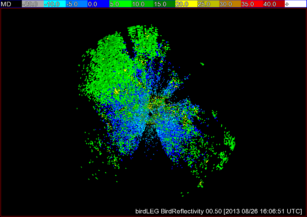
The question I want to answer: “What are the polarimetric characteristics of gust fronts”?

The methodology is to:

  1. collect a set of polarimetric radar data that have gust fronts
  2. draw polygons around the gust fronts using wg
  3. Use w2polygon2csv to extract all the pixel data within the polygons
  4. Write a R program to do linear regression of the parameters to identify gust fronts
  5. write a program to draw histograms

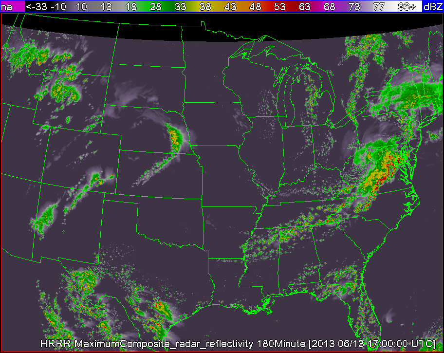
Step 1:  Data collection and ingest

I downloaded the necessary Level-II data from NCDC’s HAS website ,  untarred it and put it all in a directory named “raw”.  The directory listing looks like this.

listing
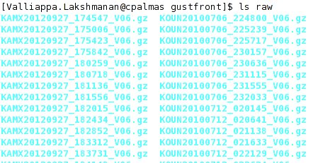
Note that I have put all the files (even those from different radars) into the same directory.

While you could ingest them all separately into separate directories for each of the radars, it is more convenient (scripting-wise) to fool downstream algorithms by pretending that all the data comes from the same radar (I’ll assume KOUN).  This is done by the following call to ldm2netcdf:

rm -rf KOUN/netcdf; ldm2netcdf -i `pwd`/raw -o `pwd`/KOUN/netcdf -s KOUN -a -1 -p gz --verbose; makeIndex.pl `pwd`/KOUN/netcdf code_index.xml

After this, you will have a directory called KOUN/netcdf within which will be netcdf files corresponding to Reflectivity, Zdr, etc.

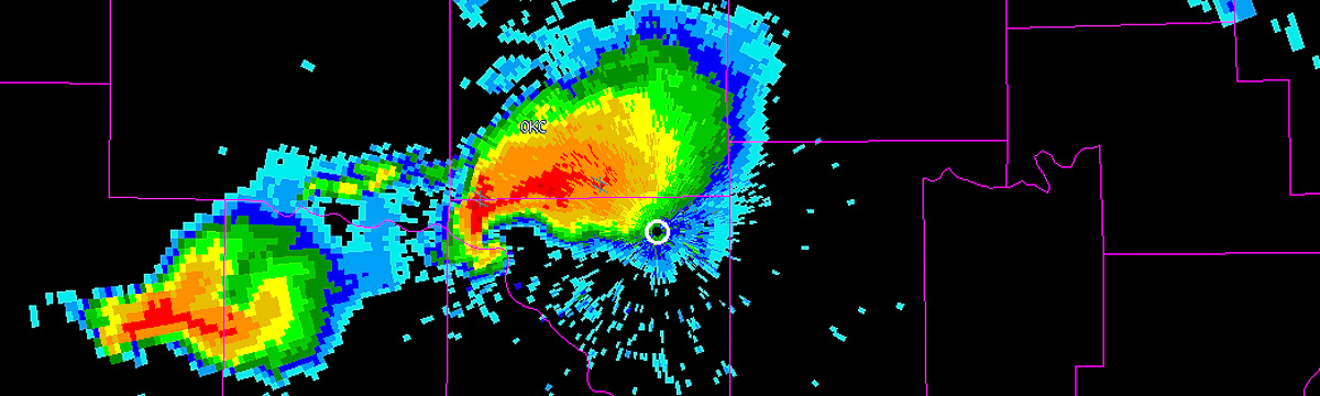
Step 2: Drawing polygons

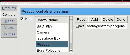
Start up wg and select Controls | Readout.  Change the output directory in the unmarked textbox (the default is probably /tmp) to the location where you want the polygon files saved:

setupBring up your data product (in this case, Reflectivity). Click on Add and then click around the gustfront to draw a polygon around the gustfront.  If you have multiple gust fronts, use the Done button to finish one polygon and start another. When you are finally done, click Save:

polygon
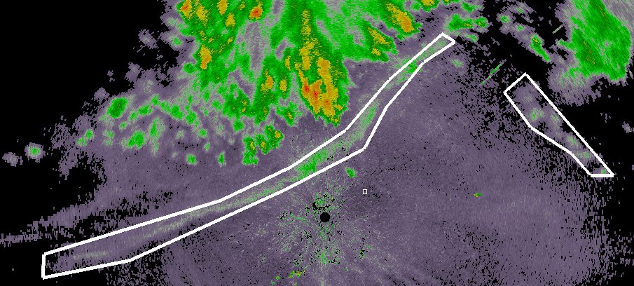
At this point, a polygon XML file is written to the output directory. It will have a name like GustFront_Reflectivity_20120709-003408.xml where GustFront is the name of the data source in wg, Reflectivity the name of the product and the rest of the filename is the time stamp.

Move to the next image, click Reset to clear the existing polygon from the display and draw the set of polygons corresponding to the new time step.  Repeat for all your data cases (you can skip time steps if you want).

Step 3: Extract pixel data using w2polygon2csv

It is helpful to extract data both from within the polygons (“gustfronts”) and from outside the polygons (“not gustfronts”).  The raw data that I want to collect are Reflectivity, AliasedVelocity, RhoHV and Zdr.  I can also collect any other data as long as I have an algorithm that will produce that data in polar format.

Run w2polygon2csv as follows:

#!/bin/sh

makeIndex.pl `pwd`/KOUN/netcdf code_index.xml

rm -rf csv; mkdir -p csv/gf csv/ngf
INPUTS="Reflectivity:00.50 AliasedVelocity:00.50 RhoHV:00.50 Zdr:00.50"
NUMINPUTS=`echo $INPUTS | wc -w`
w2polygon2csv -i `pwd`/KOUN/netcdf/code_index.xml -I "$INPUTS" -o `pwd`/csv/gf -p `pwd`/polygons -F 60 -N $NUMINPUTS --verbose
w2polygon2csv -i `pwd`/KOUN/netcdf/code_index.xml -I "$INPUTS" -o `pwd`/csv/ngf -p `pwd`/polygons -F 60 -N $NUMINPUTS -V --verbose

After the above commands are run, we will have a set of comma-separated-values (CSV) files in csv/gf corresponding to gustfronts and another set of CSV files corresponding to not-gustfronts in csv/ngf.


Step 4:  Create a Linear Regression Model to identify gustfronts

If you are using R, you should combine the two sets of files, making to sure add a new column with the value 1 for gustfront pixels and 0 for not-gustfront pixels.  Like this:

head -q csv/gf/* | head -1 | awk '{print $0",GustFront"}' > csv/train.csv
cat csv/gf/*.csv | grep -v Time | awk '{print $0",1"}'  >> csv/train.csv
cat csv/ngf/*.csv | grep -v Time | awk '{print $0",0"}' >> csv/train.csv

The very first line (head) simply carries over the column information from the original CSV files.   The reason for the “grep -v” on the second and third lines is to remove this header line from all subsequent output.  At this point, you will now have a “train.csv” with all the pixel data and you can use R’s read.csv to read it and process it.

The R program to do the linear regression:

data <- read.csv("csv/train.csv")
data <- data[ data$Reflectivity < 30, ]
data <- data[ data$RhoHV < 0.9, ]

numgustfronts <- length( data[data$GustFront > 0.5,1] )
numnegatives  <- length( data[data$GustFront < 0.5,1] )
weights <- data$RhoHV
weights[ data$GustFront > 0.5 ] <- 0.5/numgustfronts
weights[ data$GustFront < 0.5 ] <- 0.5/numnegatives

model2 <- lm( GustFront ~ abs(AliasedVelocity - 6) + ChangeInReflectivity + abs(Kdp_approx) + abs(Reflectivity - 13) + RhoHV + abs(Zdr), data=data, weights=weights )

You may notice that I have additional columns in my output — I used existing WDSS-II tools (beyond the scope of this blog) to produce a ChangeInReflectivity (over time) and to approximate the Kdp.

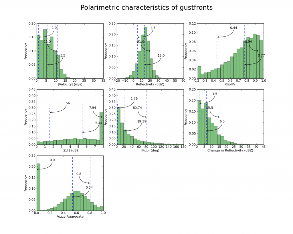
Step 5: Draw histograms using Python

You could use R itself to draw histograms, but these days, I prefer using Python, and so I will read the individual files from within the Python program itself. My Python program, for simplicity, will read and plot only the gustfront csv files (repeat for the non-gustfront data).

The first part of the Python program reads in the data:

#!/usr/bin/python
import matplotlib as mpl
import matplotlib.pyplot as plt
import numpy as np
import os

(VEL,DELREF,FZAGG,KDP,REF,RHOHV,ZDR,TIME,LAT,LON,NUMDATACOLS)=range(0,11)

PREFIX="gf"; TITLE="gustfronts"
#PREFIX="ngf"; TITLE="non-gustfronts"

indir="/scratch2/lakshman/gustfront/csv/" + PREFIX

# read all the files in the above directory ...
files = os.listdir(indir)
alldata = np.empty([0,NUMDATACOLS])
for file in files:
  try:
     # read file, but convert last-but-two element (which is time) to zero
     data = np.loadtxt(indir + "/" + file, comments="#", delimiter=",", unpack=False, skiprows=1, converters={(NUMDATACOLS-3): lambda s: 0} )
     # remove any points that do not have a valid value
     sel = data[:,0] > -999
     for col in xrange(1,NUMDATACOLS):
        sel = np.logical_and(sel, data[:,col] > -999)
     sel = np.logical_and(sel, data[:,RHOHV] < 0.99 )  # rhohv valid value < 1
     data = data[sel]
     print np.shape(data)
     alldata = np.row_stack( (alldata, data) )
  except:
     print "Ignoring " + file

As I read in the data, I append it to an array called “alldata”, so at the end of the loop, my “alldata” contains all the valid (non-missing) data in the CSV files.

The next step is to define two Python functions, one to compute the nth percentile of the data and the other to plot a nice-looking histogram:

def percentile(a, P):
  # sort a
  a = np.sort(a)
  n = int( round(P*len(a) + 0.5) )
  if n > 1:
     return a[n-2]
  else:
     return a[0]

def plothist(a, title):
  global nrows, ncols, plotno
  axes = plt.subplot(nrows,ncols, plotno)
  weights = np.ones_like(a) / len(a)
  axes.hist(a, numbins, facecolor='green', normed=False, alpha=0.5, weights=weights)
  p = percentile( np.abs(a), 0.1 )
  plt.plot( [p,p], axes.get_ylim(), 'b--' )
  pos = axes.get_ylim()[0] * 0.25 + axes.get_ylim()[1] * 0.75
  axes.annotate( np.around(p,2),
                 xy=(p, pos), xycoords='data',
                 xytext=(50,30), textcoords='offset points',
                 arrowprops=dict(arrowstyle="->",
                      connectionstyle="angle3,angleA=90,angleB=0") )
  p = percentile( np.abs(a), 0.5 )
  plt.plot( [p,p], axes.get_ylim(), 'b--' )
  pos = axes.get_ylim()[0] * 0.75 + axes.get_ylim()[1] * 0.25
  axes.annotate( np.around(p,2),
                 xy=(p, pos), xycoords='data',
                 xytext=(50,30), textcoords='offset points',
                 arrowprops=dict(arrowstyle="->",
                      connectionstyle="angle3,angleA=90,angleB=0") )
  p = percentile( np.abs(a), 0.9 )
  plt.plot( [p,p], axes.get_ylim(), 'b--' )
  axes.annotate( np.around(p,2),
                 xy=(p, np.mean(axes.get_ylim())), xycoords='data',
                 xytext=(-50,30), textcoords='offset points',
                 arrowprops=dict(arrowstyle="->",
                      connectionstyle="angle3,angleA=90,angleB=0") )
  axes.set_ylabel("Frequency")
  axes.set_xlabel(title)
  #plt.title("Distribution of " + title)
  plotno = plotno + 1

Then, simply call the histogram function once per variable:

# process the data
data = alldata
print "Total: ",np.shape(data)

plotno=1
nrows=3
ncols=3
numbins=20

plt.figure(figsize=(15,12))

plothist( np.abs(data[:,VEL]), '|Velocity| (m/s)')
plothist( data[:,REF], 'Reflectivity (dBZ)' )
plothist( data[:,RHOHV], 'RhoHV' )
plothist( np.abs(data[:,ZDR]), '|Zdr| (dB)')
plothist( np.abs(data[:,KDP]), '|Kdp| (deg)')
plothist( data[:,DELREF], 'Change in Reflectivity (dBZ)' )
plothist( data[:,FZAGG], 'Fuzzy Aggregate')

fig = plt.gcf()
fig.suptitle("Polarimetric characteristics of " + TITLE, fontsize=24)
#plt.show()
plt.savefig( PREFIX + 'stats.png') #, bbox_inches='tight')

The final output looks like this:

gfstats


Tags: None

Environmental information in w2dualpol

In order to run the hydrometer classification algorithm (HCA) and melting layer detection algorithm (MLDA) in w2dualpol, a “first guess” at the melting layer is required. Previously, the same default first guess was used for all radars. Obviously this solution is not ideal, as on any given day, the melting layer is likely to vary wildly across different radar sites (not to mention that at any given radar site, the melting layer is likely to vary wildly across different days).

For a better solution, you can now pull environmental information (specifically, the 0C wet bulb temperature height) into w2dualpol for a more realistic first guess at the melting layer. This first guess is provided through the use of a SoundingTable. The SoundingTable can be created in one of three ways: (1) The WDSS-II program nse can create this from a RUC analysis field.  (2) The ingest_sounding.pl script reads and converts sounding data from the U. Wyoming website into WDSS-II’s XML format. (3) You can write your own XML table file.

Once you have your SoundingTable, you will want to be sure that it is included in your RadarIndex. Then, in the command for w2dualpol, set the -S flag, and from there the algorithm will use the SoundingTable information to create a first guess at a melting layer. Additionally, the melting layer found from the SoundingTable will be used in instances when the data is not sufficient for the MLDA to run.

It should be noted that once the SoundingTable is greater than 1 day older than the radar data being processed, the SoundingTable will be aged off and the default melting layer will be used. On a related note, we have altered the algorithm such that if more than two hours pass after the MLDA has run, the algorithm will revert to using the melting layer found in the SoundingTable.

A few final notes; If a SoundingTable is present in the RadarIndex but you do not wish to use it, set -S junk and the default value will be used for the melting layer. Additionally, if no SoundingTable is available, there is no need to set -S.

Tags: None

User defined resolution in w2birddensity

A secondary use of weather radars is to detect biological scatterers such as birds, bats, and insects. When birds are detected, the echoes returned to the radar can be used to estimate the density of birds on the ground. This information is valuable in a number of situations, such as when attempting to determine where birds stop while in their migratory journey.

The algorithm w2birddensity, which is based on an algorithm described in detail here, estimates the bird density from radar reflectivity data. This is done by computing a vertical profile of reflectivity (VPR) and making adjustments to the raw reflectivity field based off of the VPR.

Previously, w2birddensity was carried out at a fixed resolution, but we have now given users the option of defining the resolution of their radar data with the -R flag. As with many of our other algorithms, just specify the gate size in km, the radial size in degrees, and the range in km, as shown below. Additionally, we have given the user the option of specifying that they would like more then the default of 5 tilts processed. This is done by setting the -n flag to the number of tilts desired.

w2birddensity -i /localdata/birddensity/code_index.xml -o /tmp/birds -s KAKQ -E ~/WDSS2/gtopo30/radars -R 0.25x0.5x100 -n 5 --verbose
birdSR
Bird reflectivity from KIWA at super-resolution.
BirdLEG
Bird reflectivity from KIWA at legacy resolution.


Tags: None